Chandrayaan-2 XSM
Solar X-ray Monitor
This website provides only the plots of solar X-ray flux integrated over either the GOES XRS-B energy range (1-8 Å or 1.55 to 12.4 keV) or the full XSM energy range (1 - 15 keV), obtained from the XSM spectra. Full spectral data is available in the data archive. The raw (level-1) and calibrated (level-2) XSM data organized into day-wise files are available for download from the PRADAN portal of ISRO Science Data Archive (ISDA) at Indian Space Science Data Center (ISSDC), Bangalore.
To dowload the data, visit https://pradan.issdc.gov.in/ch2/. Users need to register in the website for accessing the data.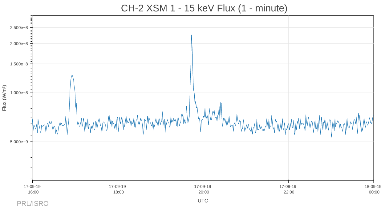
mithun@Thinkpad:xsm_analysis$ unzip ch2_xsm_20190917_v1.zip
This will create a directory structure with xsm as top level directory with year, month, day
level sub-directory structure under data as:
xsm/
   data/
       2019/
           09/
             17/
              raw/
                 ch2_xsm_20190917_v1_level1.fits
                 ch2_xsm_20190917_v1_level1.hk
                 ch2_xsm_20190917_v1_level1.sa
              calibrated/
                 ch2_xsm_20190917_v1_level2.gti
                 ch2_xsm_20190917_v1_level2.pha
                 ch2_xsm_20190917_v1_level2.lc
| Period | Tstart | Tstop |
| Flare | 85520490.0 (19:41:30) | 85520850.0 (19:47:30) |
| Non-flaring | 85527600.0 (20:40:00) | 85534800.0 (23:40:00) |
mithun@Thinkpad:~/xsm_analysis/xsm/data/2019/09/17/calibrated$ xsmgenspec
-------------------------------------------------------------------------
  XSMDAS: Data Analysis Software for Chandrayaan-II Solar X-ray Monitor
                     XSMDAS Version: 1.1
                     Module : XSMGENSPEC
-------------------------------------------------------------------------
Enter Input Level-1 file [] : ../raw/ch2_xsm_20190917_v1_level1.fits
Enter Output Spectrum file [] : ch2_xsm_20190917_flare.pha
Enter output spectrum type  [time-resolved] : time-integrated
Enter start time for extracting spectrum [0] : 85520490.0
Enter stop time for extracting spectrum [0] : 85520850.0
Enter HK file [] : ../raw/ch2_xsm_20190917_v1_level1.hk
Enter Sun angle file [] : ../raw/ch2_xsm_20190917_v1_level1.sa
Enter GTI file [] : ch2_xsm_20190917_v1_level2.gti
------------------------------------------------------------------------
MESSAGE: Ebounds CALDB file used is: /home/mithun/work/ch2/xsm/pipeline/XSM/xsmdas/caldb/CH2xsmebounds20191214v01.fits
MESSAGE: Gain CALDB file used is: /home/mithun/work/ch2/xsm/pipeline/XSM/xsmdas/caldb/CH2xsmgain20200330v03.fits
MESSAGE: Abscoef CALDB file used is: /home/mithun/work/ch2/xsm/pipeline/XSM/xsmdas/caldb/CH2xsmabscoef20200410v01.fits
MESSAGE: Effareapar CALDB file used is: /home/mithun/work/ch2/xsm/pipeline/XSM/xsmdas/caldb/CH2xsmeffareapar20200410v01.fits
MESSAGE: Syserror CALDB file used is: /home/mithun/work/ch2/xsm/pipeline/XSM/xsmdas/caldb/CH2xsmsyserr20200410v01.fits

MESSAGE: XSMGENSPEC completed successully
MESSAGE: Output file = ch2_xsm_20190917_flare.pha
MESSAGE: Output ARF = ch2_xsm_20190917_flare.arf
At the end of execution a spectrum file and arf file will be generated. Similarly generate
spectrum and arf for the non-flaring duration by providing appropriate start and stop times.
Before proceeding to detailed spectral analysis, load both these spectra in XSPEC with a sample
background file provided under $xsmdas/caldb/bkgspec as the background spectra (either copy
the background pha to present working directory or give full path) using appropriate XSPEC
commands as below:
XSPEC12>da 1:1 ch2_xsm_20190917_flare.pha

1 spectrum  in use

Spectral Data File: ch2_xsm_20190917_flare.pha  Spectrum 1
Net count rate (cts/s) for Spectrum:1  1.438e+01 +/- 2.307e-01
 Assigned to Data Group 1 and Plot Group 1
  Noticed Channels:  1-512
  Telescope: CH-2_ORBITER Instrument: CH2_XSM  Channel Type: PI
  Exposure Time: 360 sec
 Using fit statistic: chi
 Using test statistic: chi
 Using Response (RMF) File    /home/mithun/work/ch2/xsm/pipeline/XSM/xsmdas/caldb
/CH2xsmresponse20200423v01.rmf for Source 1
 Using Auxiliary Response (ARF) File  ch2_xsm_20190917_flare.arf

XSPEC12>back 1 ch2_xsm_20191128_bkg.pha
Net count rate (cts/s) for Spectrum:1  1.324e+01 +/- 2.307e-01 (92.1 % total)
XSPEC12>da 2:2 ch2_xsm_20190917_post-flare.pha

2 spectra  in use

Spectral Data File: ch2_xsm_20190917_post-flare.pha  Spectrum 2
Net count rate (cts/s) for Spectrum:2  7.242e+00 +/- 7.831e-02
 Assigned to Data Group 2 and Plot Group 2
  Noticed Channels:  1-512
  Telescope: CH-2_ORBITER Instrument: CH2_XSM  Channel Type: PI
  Exposure Time: 7200 sec
 Using fit statistic: chi
 Using test statistic: chi
 Using Response (RMF) File    /home/mithun/work/ch2/xsm/pipeline/XSM/xsmdas/caldb
/CH2xsmresponse20200423v01.rmf for Source 1
 Using Auxiliary Response (ARF) File  ch2_xsm_20190917_post-flare.arf

XSPEC12>back 2 ch2_xsm_20191128_bkg.pha
Net count rate (cts/s) for Spectrum:2  6.100e+00 +/- 7.840e-02 (84.2 % total)
Plot the spectra after ignoring the data below 1 keV and above 5 keV using ignore, plot, and setplot commands in XSPEC (see XSPEC manual). Figure below shows the resulting plot. The black data points denote the flare spectrum, red data points correpond to non-flaring period spectrum and the stars denote the background spectra.
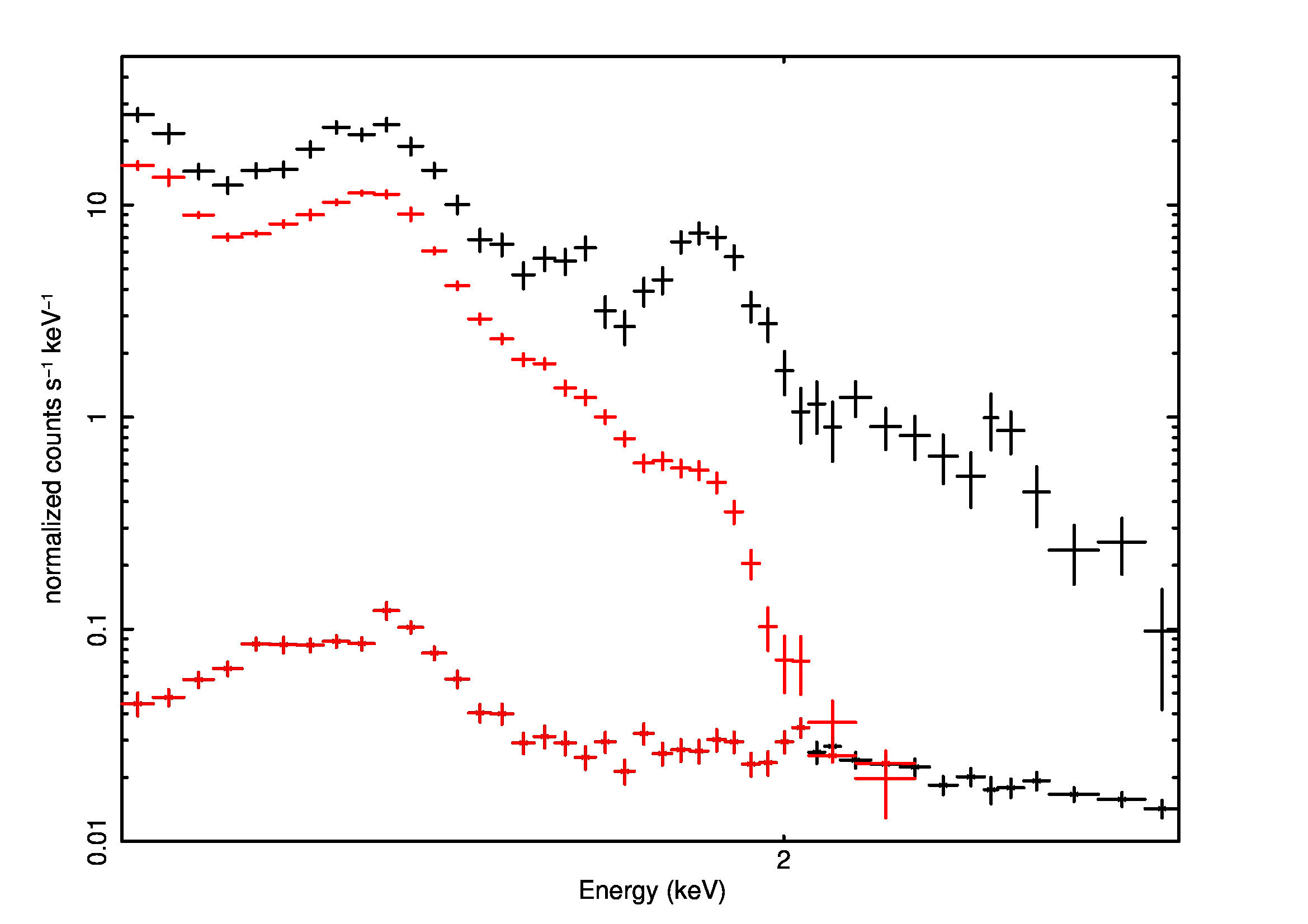
As noted in caveats below, background in XSM shows slight variability and thus it is recommended to restrict the spectral analysis to energies where the source is well above background. In this example, we shall choose non-flaring spectrum up to 2.3 keV and flare spectrum up to 2.7 keV for spectral fitting. We also need to ignore the spectra below 1.3 keV as noted in the caveats (this observation is before June 2020).
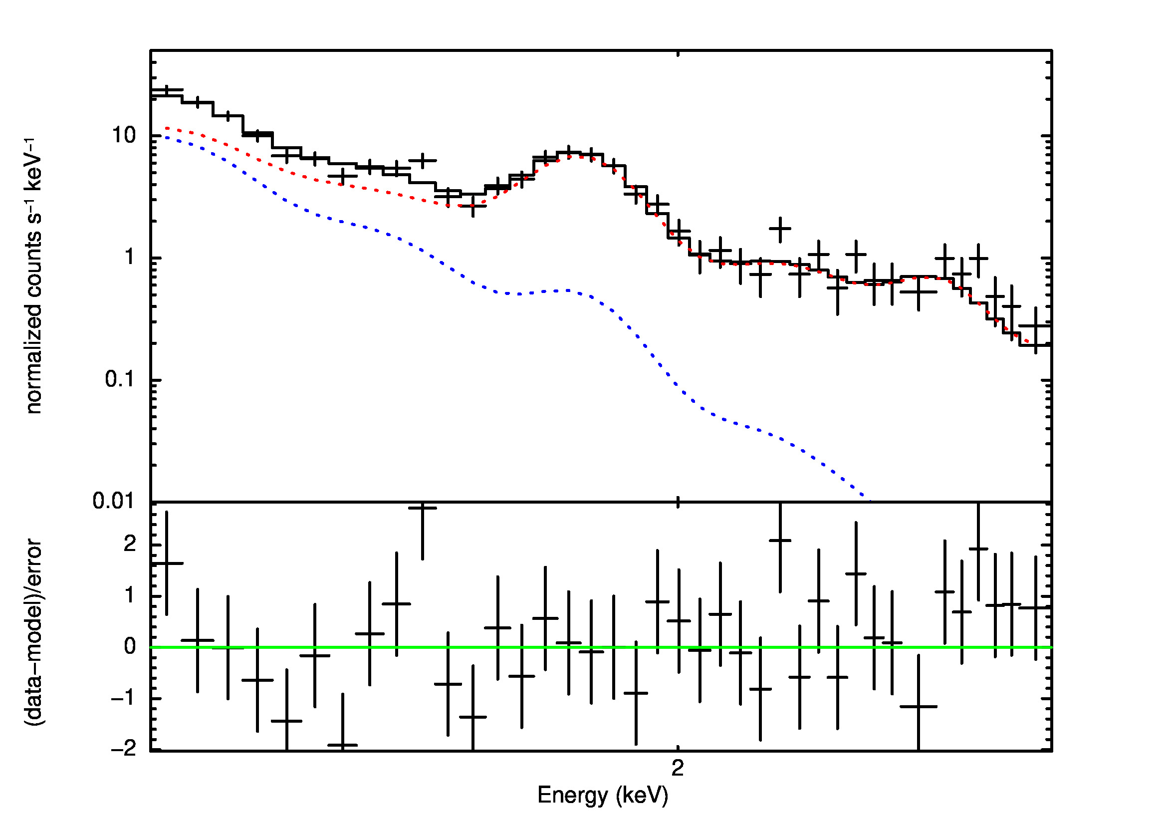
First, we fit the pre-flare spectrum with an isothermal plasma emission model vapec. The abundances shall be set to typical solar coronal abundances and that of elements Mg, Al, and Si shall be left free while fitting. Refer to XSPEC manual for the steps involved. We then fit the flare spectrum by using a two temperature model, as the sum of two vapec models. The parameters of the first component is frozen to that obtained for pre-flare duration whereas the parameters of the second component are left free. Flare spectrum with the best fit two-component model is shown in the below figure for reference.
To load the XSM spectral data (level-2 time-series PHA file) and response in OSPEX, two
IDL routines are provided along with the XSMDAS distribution (see the directory $xsmdas/idl).
Add this location to IDL PATH or copy the two IDL rouines named ch2xsm_read_data.pro and
ch2xsm_read_drm.pro to any of the pre-defined IDL PATH locations, so that they are accessible
by SolarSoft. It may be noted that these routines are not meant to be used independant of
OSPEX.
For XSM data analysis with OSPEX, start SSW IDL session and invoke OSPEX as:
o=ospex()
This will open up a window of OSPEX GUI. Then, set the spex file reader to the XSM data read routines as:
o->set, spex_file_reader='ch2xsm_read'
Then, use File -> Select Input option in the GUI to load the standard
time-resolved spectrum file (60 s cadence) available under the calibrated directory into OSPEX.
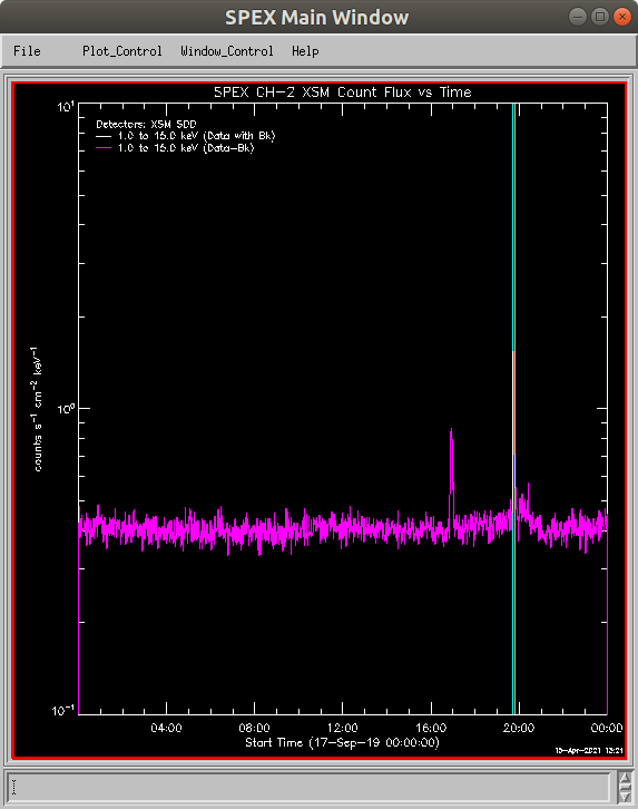
After loading the file, on clicking plot time profile option, OSPEX window will plot the light
curves in different energy bands as shown below.
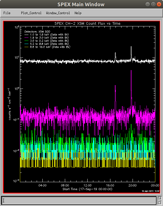
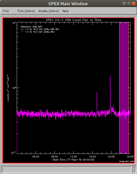
For analysis of flare spectrum, we need to select a flare time interval and a non-flaring time interval (as background) using the select time interval options in the OSPEX window. An example of flare and background time selection is shown below.
After the selection, on plotting the spectrum for the selected flare duration, window will show the spectrum as below where the fitting interval is selected as 1.3-3.0 keV.
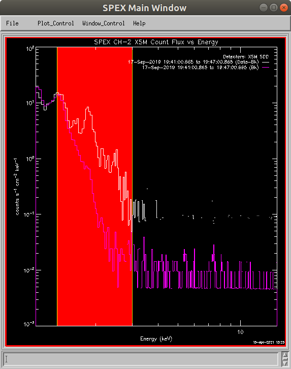
Now, one can proceed to fit the spectrum with available models in OSPEX, suitable one being
vth_abun.
| Version | Release Date | Notes |
| 1.1 | 10 Dec 2020 | First public release |
| 1.2 | 28 Jun 2021 | Included python script for computing flux over a user provided energy range; CALDB version used are written in output spectra/resp/lc headers. |
| 1.5 | 21 Nov 2025 | Incorporated proper deadtime correction model, the exposures of generated spectrum are corrected with the deadtime model. Generates response with Beryllium filter for large flare. Recent version of cfitsio library included with the software for compatibility with latest Mac OS versions.Bug fixes for latest apple gcc compilers are included. |
| Version | Release Date | Notes |
| 20201210 | 10 Dec 2020 | First public release |
| 20210628 | 28 Jun 2021 | Added new gain file for observations from June 2020 with new LLD setting and updated effective area parameters for N-M season |
| 20251111 | 11 Nov 2025 | Includes a new lookup table for deadtime correction, compatible with XSMDAS V1.5 |