Chandrayaan-3 APXS
Alpha Particle X-ray Spectrometer
The raw (level-1) and calibrated (level-2) APXS data for each observation are available for download from the PRADAN portal of ISRO Science Data Archive (ISDA) at Indian Space Science Data Center (ISSDC), Bangalore. For measured abundance values, please refer to Vadawale et al (2024, Nature).
To dowload the data, visit https://pradan.issdc.gov.in/ch3/. Users need to register in the website for accessing the data.
Users are requested to acknowledge the use of APXS data and analysis software by citing the relevant publications as well as by including the following statement in acknowledgment:
"We acknowledge the use of data from the APXS instrument on the rover of the Chandrayaan-3 mission of the Indian Space Research Organisation (ISRO), archived at the Indian Space Science Data Centre (ISSDC). APXS experiment is designed and developed by the Physical Research Laboratory (PRL), Ahmedabad with support from Space Applications Center (SAC), Ahmedabad and U.R Rao Satellite Center (URSC), Bangalore."
APXS measured the X-ray fluorescence spectra from the lunar surface. Calibrated data of APXS includes the X-ray spectrum file in standard PHA format and instrument response matrix. In order to obtain elemental abundances from the observed X-ray spectra, they are to be fitted with lines corresponding to individual elements. From the measured line fluxes, abundances can be estimated using the correlations obtained during ground calibration. The detailed procedure of obtaining the correlations from ground calibration data with geo-chemical reference samples and using these correlations to obtain abundances from measured line fluxes is given in Mithun et al (2020, PSS).
The APXS team have analysed the X-ray spectra at each rover stop and the results of this is reported in Vadawale et al (2024, Nature). Interested users may use those abundance measurements for their scientific interpretations and may not be required to carry out the analysis as outlined below for abundance measurements.
However, for interested users, a brief overview of the procedure to obtain abundances from APXS spectra is given here and they are directed to Mithun et al (2020, PSS) and Vadawale et al (2024, Nature) for more details.
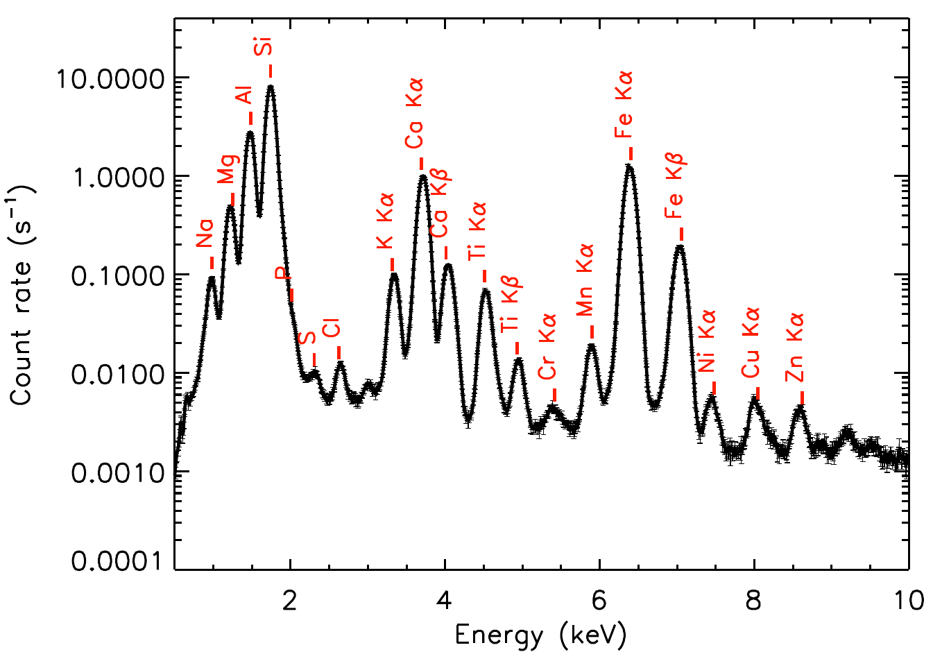
Figure below shows the APXS spectrum of a geo-chemical reference sample W-2A where the lines from different elements are identified. It may be noted that this spectrum is obtained for a long exposure of 15 hours whereas the typical exposures for lunar samples will be around 45 minutes. Similar spectrum, with different lines at different intensities, are expected for lunar samples. By comparing the energy of observed lines with K-α K-β energies of various elements, elements present can be identified.
Once the elemental lines are identified, the spectrum is to be fitted with model of multiple lines and a continuum to obtain the line fluxes. As the instrument’s spectral response also needs to be taken into account, it is recommended to use the standard X-ray spectral fitting package XSPEC, which takes care of this internally if the files in proper formats are given. Refer XSPEC user manual for more details on XSPEC spectral analysis. APXS spectra and response files are compatible with XSPEC and can be loaded easily for perform spectral fitting. However, users may chose to use other fitting programs for obtaining line fluxes taking into account the spectral redistribution matrix.
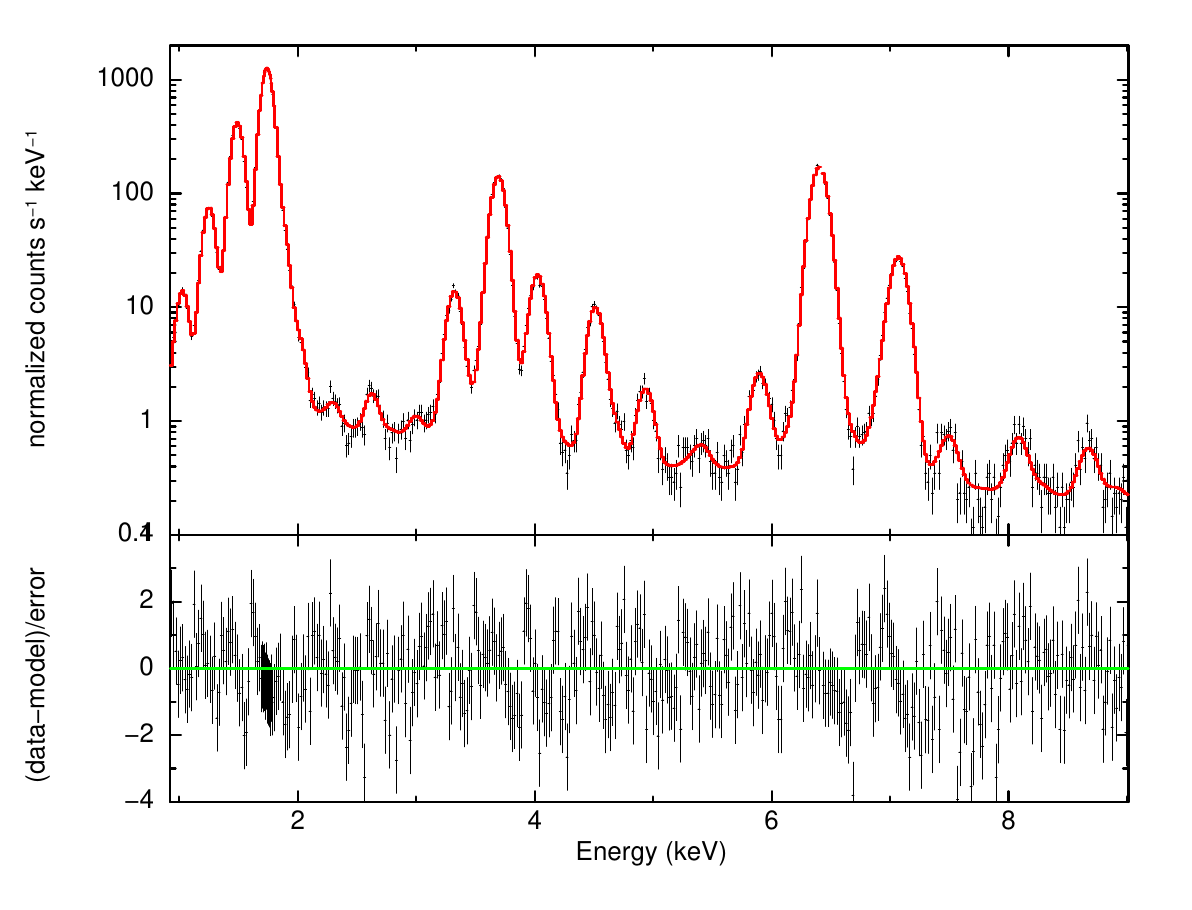
The figure below shows a typical sample spectrum for 45 minute exposure fitted with multiple lines (Gaussians with zero width) and a continuum consisting of broken power-law models in XSPEC. Once all observed lines are accounted for in the model, a satisfactory fit with minimal residuals can be obtained as shown in the figure. The line fluxes obtained from the best fit are then to be used to get abundance values.
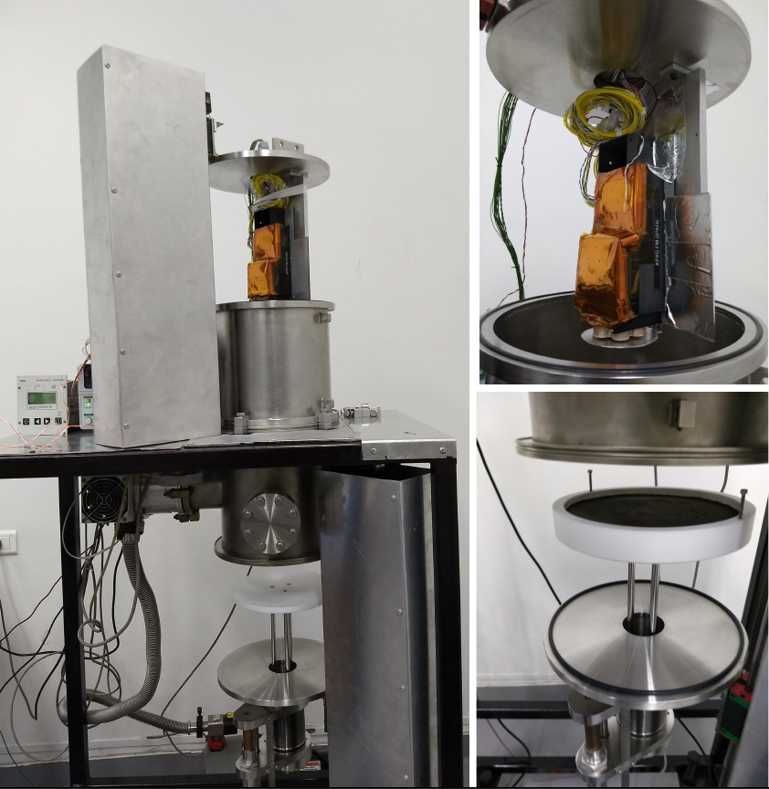
In order to develop conversion from the observed line intensities to abundances, detailed ground calibration was carried out. APXS spectra were obtained for a suite of geo-chemical reference materials with known composition and the measured line intensities were correlated with the abundances. Line intensity of a particular element often depends on the abundance of other elements as well and this is termed as matrix effect. Thus the correlations are obtained after incorporating matrix corrections to the measured line intensities as described in Mithun et al (2020, PSS). The images below shows the vacuum chamber setup used for obtaining the ground calibration data for APXS, by keeping the samples at different distances from the instrument.
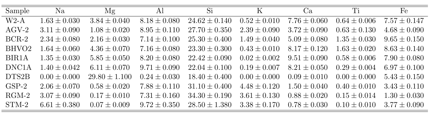
A suite of ten geochemical samples from USGS spanning the expected abundance ranges of various elements in lunar highlands were selected for the ground calibration. The table below lists these samples and their known standard abundance values.
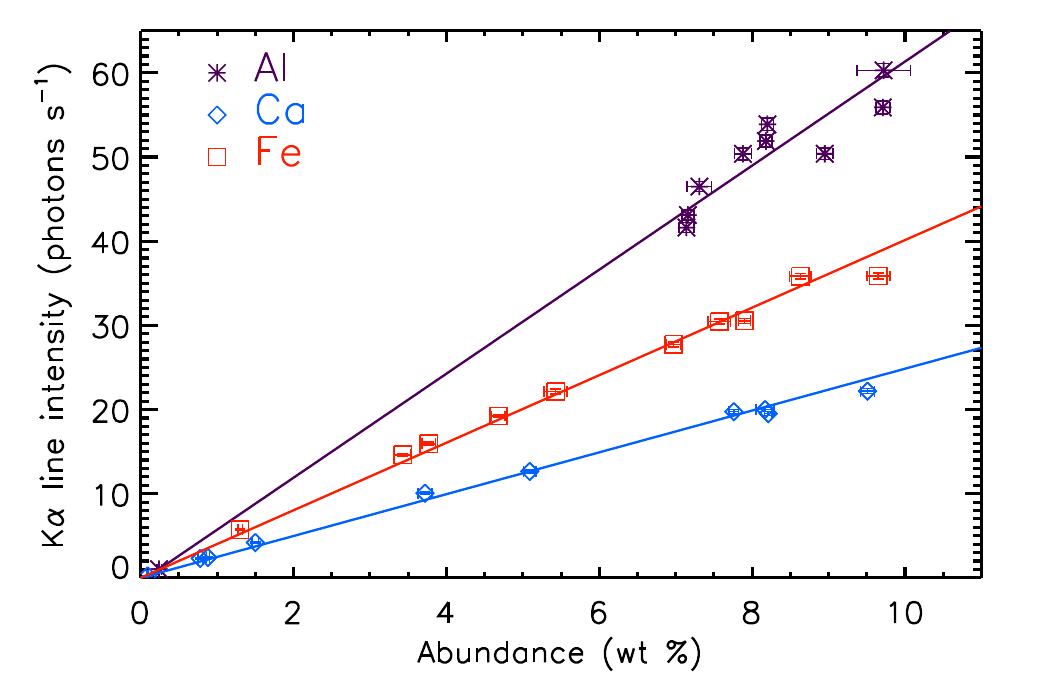
Analysing the APXS data of the USGS samples, correlations between known abundance values and measured line intensities are obtained, similar to the example shown in the figure below. It maybe noted that this figure is for the data acquired for the APXS instrument flown on Chandrayaan-2 mission. As the line intensities crucially depend on the exact source characteristics, data were also acquired with the instrument flown on Chandrayaan-3 mission and following the similar procedure, line intensity - abundance correlations are obtained. These are presented in Vadawale et al (2024, Nature).
Now for an unknown sample's X-ray spectrum, such as that of the lunar surface samples, we start with the measured line intensities of all detected elements and obtain the initial estimate of abundances using the calibration curves. Oxygen abundances are estimated considering stoichiometry and the abundances are normalized. These abundance estimates are then used to compute the matrix correction factors to the original line intensities and corrected line intensities are then used in abundance estimation in the next iteration. This process is repeated until the difference between the abundance estimates of the current and previous iterations are minimal and the final estimates of abundances are obtained. Errors on abundances can be estimates from the statistical uncertainties of the line intensity measurement as well as the systematic uncertainties of the abundance-intensity correlations.